In our proposed workflow, we put a lot of emphasis on the plate design and management. The plate will carry all information needed not only for bioanalytical purposes, but also the pharmacokinetic information needed for the study.
Plate generation, reusing and managing plates
plate <- generate_96()
plot(plate)
#> Plate not registered. To register, use register_plate()
#> Warning: Removed 96 rows containing missing values or values outside the scale range
#> (`geom_text()`).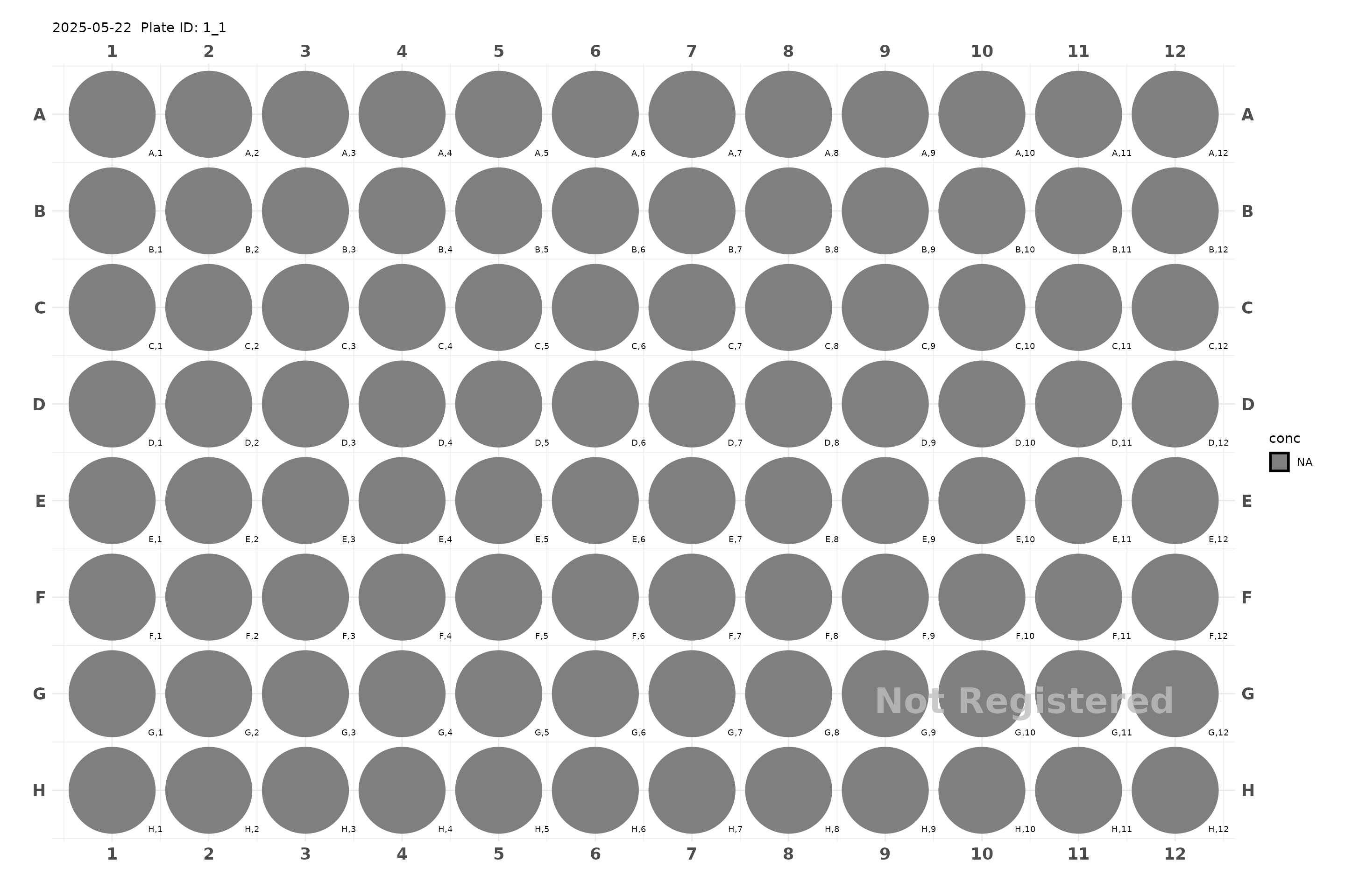
PKbioanlysis has simple database management system to keep track of the plates you have generated. After designing statistisfactory plate, you can register it in the database. After that you can generate injection sequences and dilution schemes.
You can always use print() on the created plate to see
the metadata associated with it.
print(plate)
#> 96 Well Plate
#>
#>  Active Rows: A B C D E F G H
#>  Last Fill: A,1
#>  Remaining Empty Spots: 96
#>  Description:
#>  Last Modified: 2026-06-23 16:02:36.580149
#>  Scheme h
#>  Plate ID: 1_1
#>  Registered: FALSE
#> NULL
Plate name can be specified during plate generation
generate_96(descr = "plate1") or modified by using
plate_metadata(plate, descr = "plate1").
The first part of the plate ID is unique to the plate itself, while
the second part indicated the reuse of the plate. You can reuse the
plate by calling reuse_plate(plate_id). 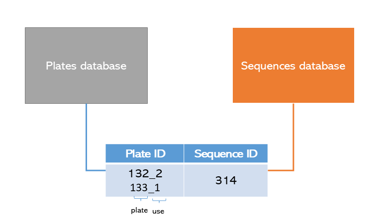
To find all previous plate, you can use study_app() to
find it and retrieve it for reuse.
Calibration study examples
plate <- generate_96("Calibration study") |>
    add_cs_curve(c(1, 3, 5, 10, 20, 50, 100, 200, 500)) |>
    add_DB() |>
    add_DB() |>
    add_blank() |>   # CS0IS1
    add_suitability(conc = 20) |>
    add_QC(2, 200 ,400, qc_serial = FALSE) |>
    add_DB() |>
    add_blank(analyte = TRUE, IS = FALSE) |> # CS1IS0
    add_cs_curve(c(1, 3, 5, 10, 20, 50, 100, 200, 500)) |>
    add_QC(2, 180 , 400, group = "test")

plot(plate, label_size = 1)
#> Plate not registered. To register, use register_plate()
#> Warning: Removed 48 rows containing missing values or values outside the scale range
#> (`geom_text()`).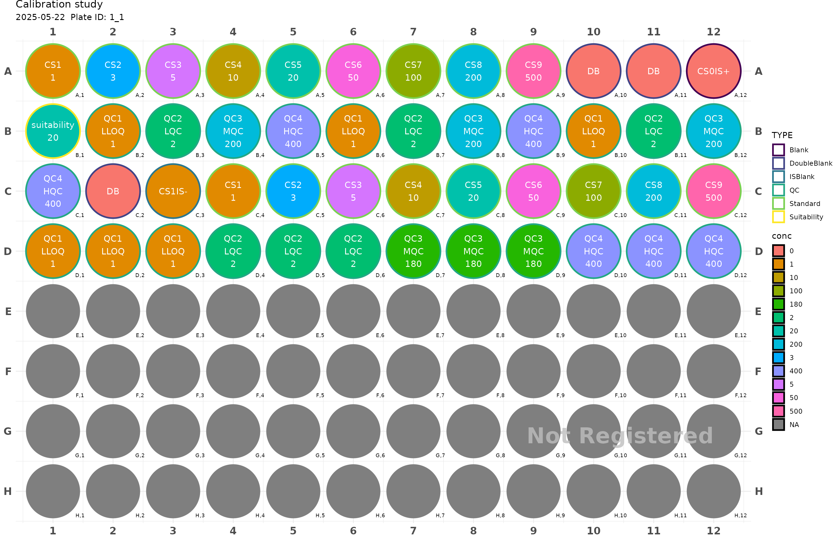
plate <- register_plate(plate)
plot(plate)
You can use make_calibration_study() for typical
calibration study instead of using add_cs_curve() and
add_QC().
plate <- generate_96() |>
    add_suitability(conc = 10) |>
    make_calibration_study(
        plate_std = c(1, 3, 5, 10, 20, 50, 100, 200, 500),
        lqc_conc = 2,
        mqc_conc = 200,
        hqc_conc = 400,
        n_qc = 4,
        qc_serial = TRUE,
        n_CS0IS0 = 2,
        n_CS1IS0 = 2,
        n_CS0IS1 = 2)
plot(plate)
#> Plate not registered. To register, use register_plate()
#> Warning: Removed 64 rows containing missing values or values outside the scale range
#> (`geom_text()`).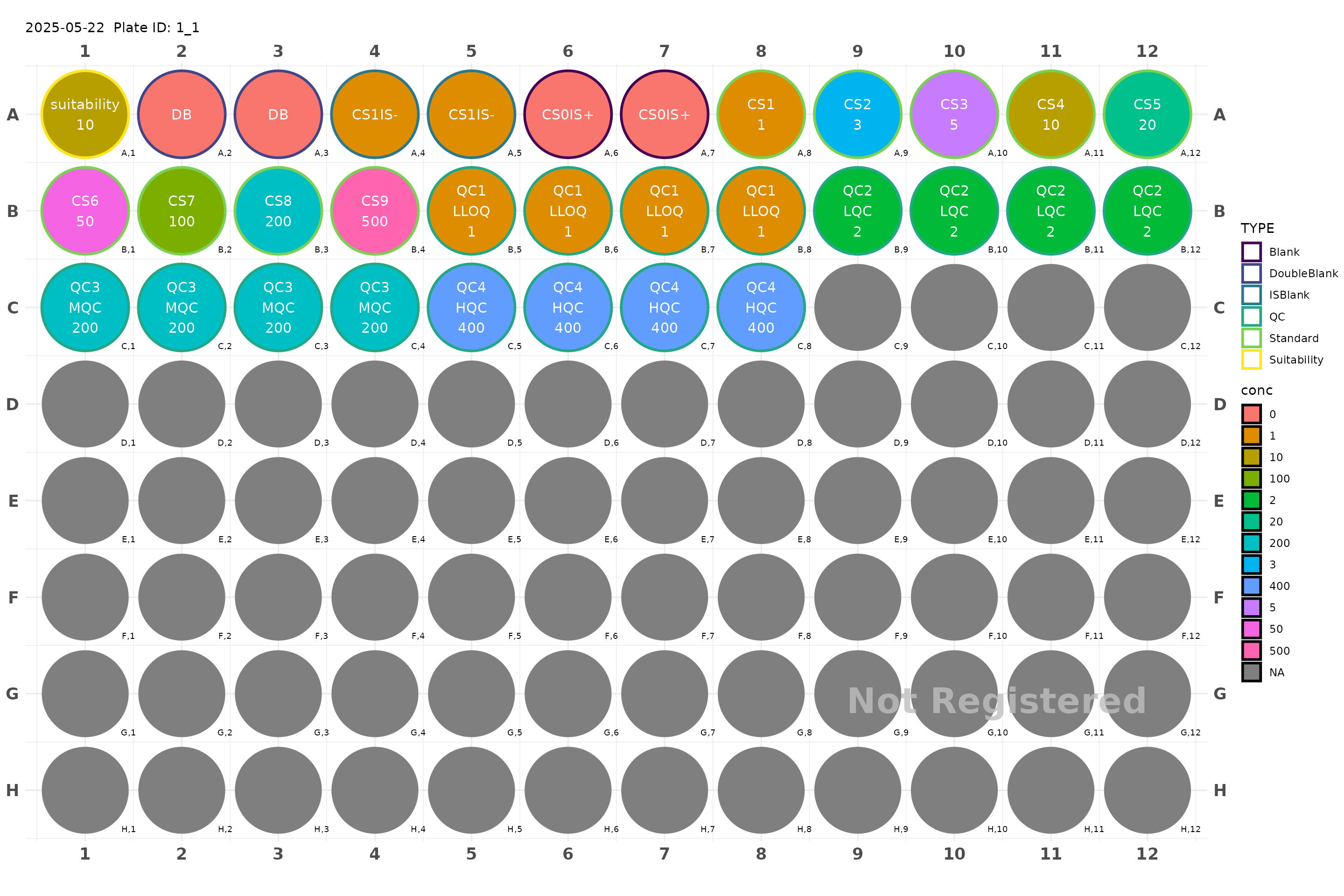
After you are satisfied with the design, you can register the plates in the database.
plate <- register_plate(plate)Finally, you can use study_app() to further inspect the
plates or to generate injection sequences and dilution schemes.
Adding samples with pharmackinetic information
PKbioanalysis offers multiple ways to add samples to plate. We
recommend having external spreadsheet with the pharmacokinetic data in
it, and then use add_samples() to add the samples with
vtime = TRUE to the plate.
Current supported pharmacokinetic information are: - Sample ID - dose - Route - CMT - Time - Factor (i.e strata)
You might also specify the dilution factor for each sample with
dil.
plate <- generate_96() |> add_samples(1:20)
plot(plate)
#> Plate not registered. To register, use register_plate()
#> Warning: Removed 95 rows containing missing values or values outside the scale range
#> (`geom_text()`).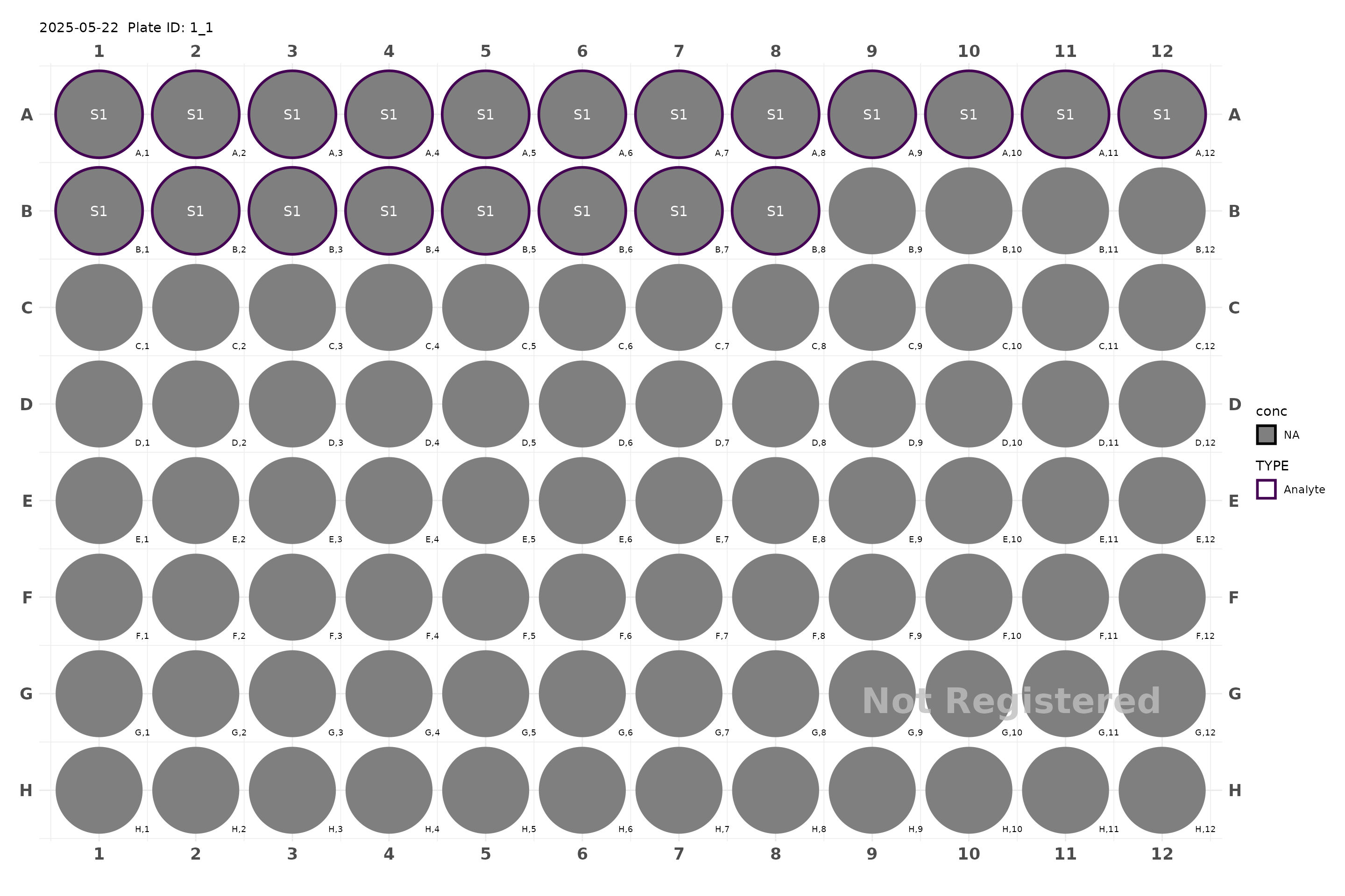
Adding samples manually
plate <- generate_96()

plate <- plate |>
    add_samples(samples = c("subject1", "subject2", "subject3"))

plot(plate)
#> Plate not registered. To register, use register_plate()
#> Warning: Removed 95 rows containing missing values or values outside the scale range
#> (`geom_text()`).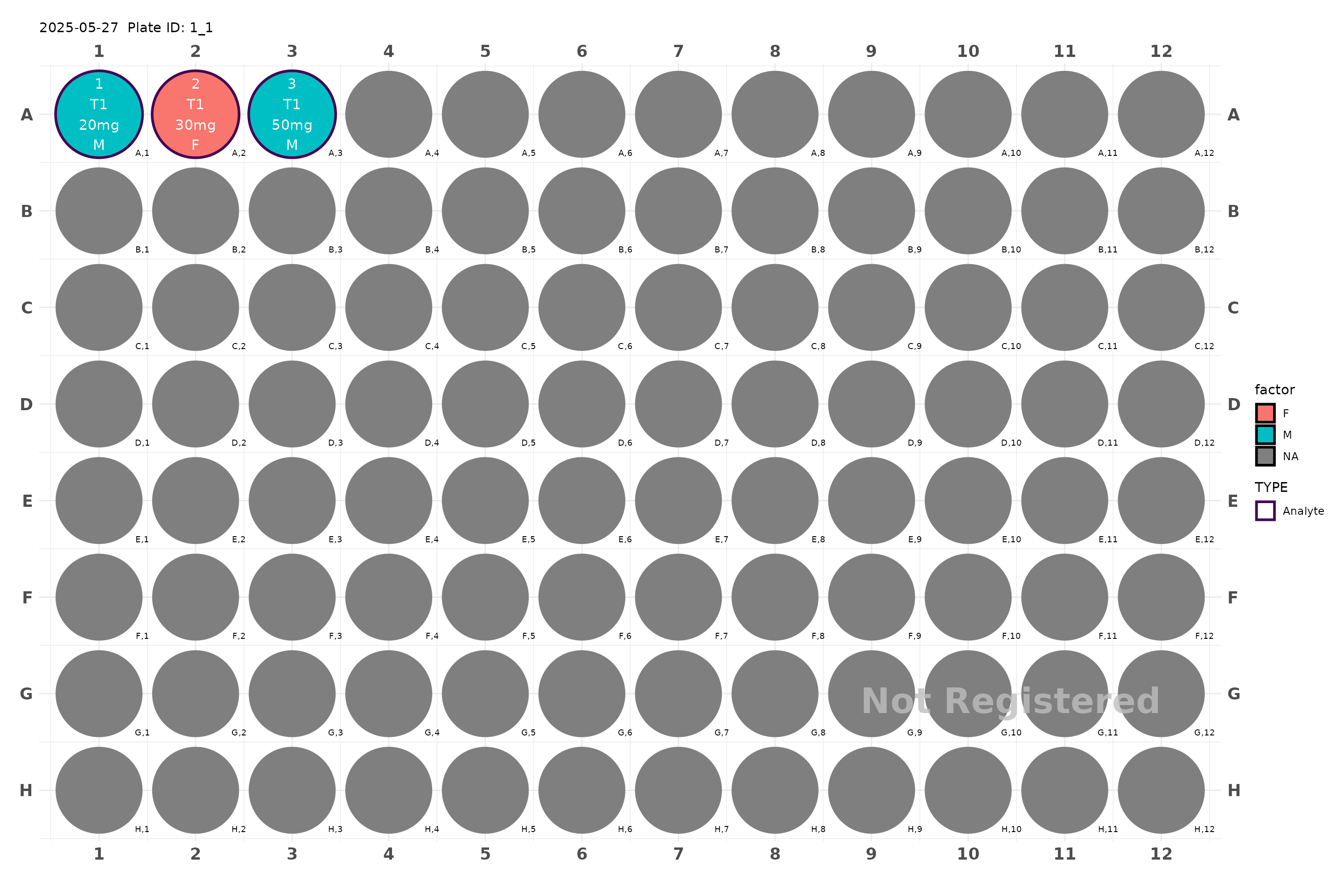
Adding samples from external spreadsheet by pharmacokinetic data
In this example, will will pass pharmacokinetic data to
add_samples(). In this case, we don’t need to repeat time
for each sample, hence we set vtime = TRUE.
data(Indometh)
plate <- generate_96() |>
    add_samples(samples = Indometh$Subject,
                time = Indometh$time, vtime = TRUE)
plot(plate, color = "time")
plot(plate, color = "samples")
Time propagated automatically for each subject.
plate <- generate_96() |>
    # add_samples_c(c("subject1", "subject2"), time = c(0, 10, 30, 60, 120), factor = "Male") |>
    add_samples("subject1", time = c(0, 10, 30, 60, 120),
                  factor = "Male") |>
    add_samples("subject2", time =   c(0, 10, 30, 120),
                  factor = "Female")

plot(plate, color = "time")
plot(plate, color = "samples")
plot(plate, color = "factor")
plot(plate, color = "conc")More advanced filling layouts
You might wish to position your samples in specific location on the plate, also you might want to fill either horizontally or vertically.
plate2 <- generate_96("Dilution integerity") |>
  add_DB() |>
  add_blank() |>
  add_blank() |>
  fill_scheme("h", lbound = 4, rbound = 11) |>
  add_cs_curve(c(1, 3, 5, 10, 20, 50, 100, 200), rep =3) |>
  fill_scheme("h", tbound = "D", bbound = "E", lbound = 1, rbound = 12) |>
  add_QC(3, 90, 180, reg = T, n_qc = 6, qc_serial = F) |>
  fill_scheme("h", lbound = 1, rbound = 4) |>
  add_DQC(conc = 1000, 100, rep = 6) |>
  fill_scheme("h", lbound = 1, rbound = 8) |>
  add_cs_curve(c(1, 4, 6, 8, 15, 75, 150, 200)) |>
  fill_scheme("h", tbound = "G", bbound = "H", lbound = 1, rbound = 8) |>
  add_QC(3, 95, 190, reg = T, n_qc = 4, qc_serial = F, group = "test") |>
  fill_scheme("v", lbound = 9, rbound = 12, tbound = "F", bbound = "H") |>
  add_DQC(conc = 1000, 10, rep = 6) |>
  add_DQC(conc = 1000, 100, rep = 6)
plot(plate2)
#> Plate not registered. To register, use register_plate()
#> Warning: Removed 3 rows containing missing values or values outside the scale range
#> (`geom_text()`).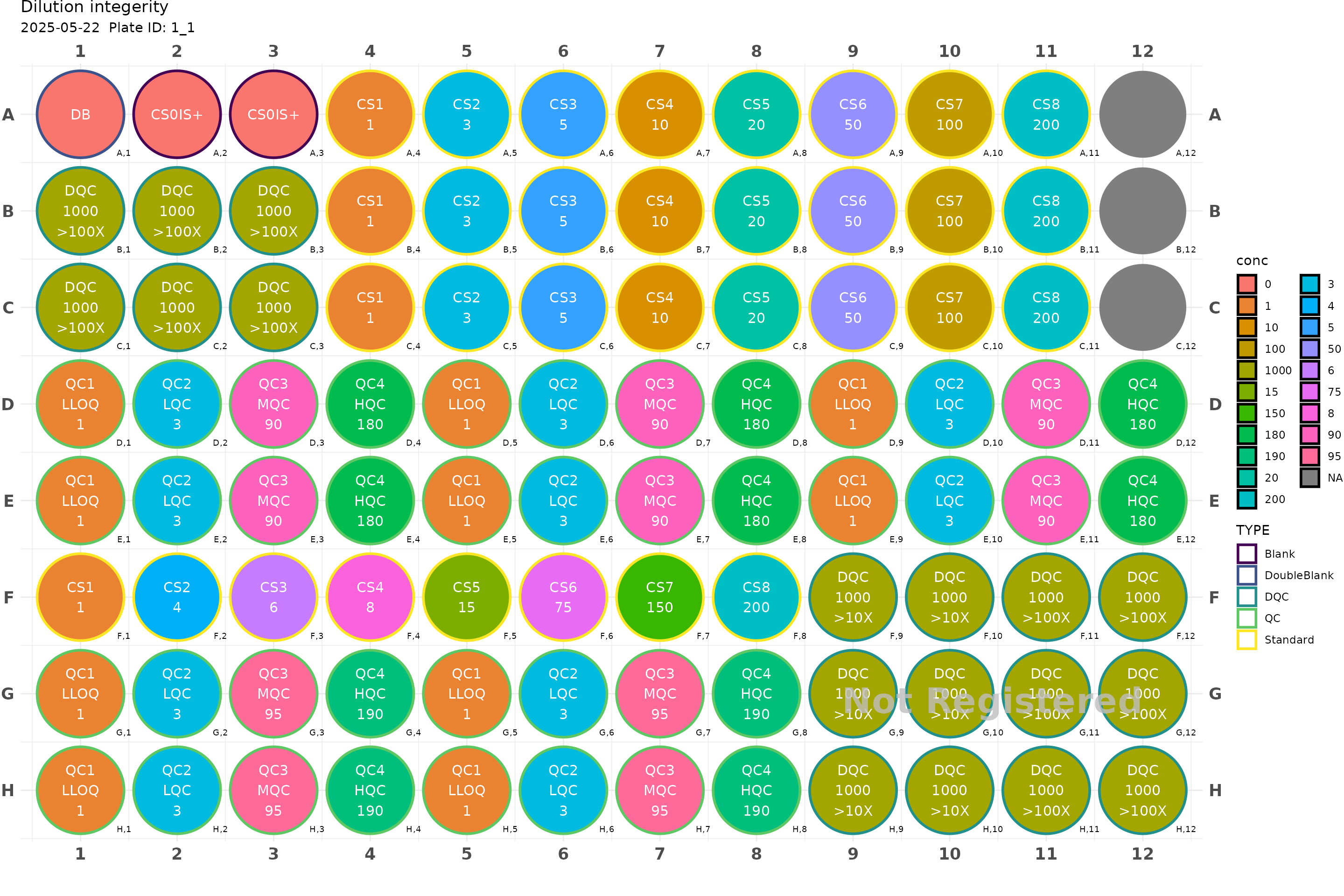
Metabolic study (Multiple plates)
plates <- make_metabolic_study(
    cmpd = c("NE", "DA", "5HT", "HVA",
             "DOPAC", "MHPG", "5HIAA", "VMA"),
    time_points = c(0, 5, 10, 15, 30, 45, 60, 90, 120),
    n_NAD = 3,
    n_noNAD = 2
)
#> ℹ Created study with ID: 6a2ac52f-250a-455b-9df0-fe06e70059ca
#> ℹ Adding dosing and subjects information...
#> ✔ Dosing information added.
#> ℹ Adding subjects information...
#> ✔ Subjects information added.
#> ℹ Adding sample log information...
#> ✔ Sample log information added.
length(plates)
#> [1] 8
plot(plates[[1]], color = "samples", label_size = 1)
plot(plates[[2]], color = "samples", label_size = 1)
plot(plates[[3]], color = "samples", label_size = 1)
plot(plates[[4]], color = "samples", label_size = 1)
plot(plates[[5]], color = "samples", label_size = 1)
plot(plates[[6]], color = "samples", label_size = 1)
register_plate(plates)