Advanced exploratory visualization techniques using ggplot2, plotly and purrr

@rinpharma 2023

Omar Elashkar

2023-10-27

Outline

  • Datasets Overview
    • Warfarin PK/PD data
  • ggplot2 Examples
  • interactive plots with plotly
  • leveraging purrr
  • 6 exercises: 5 minutes each

Material

Dataset Summary

head(war_pk)
  id time amt   dv dvid evid   wt age  sex wt_cat age_cat
1  1  0.5 100  0.0   cp    0 66.7  50 male low wt old age
2  1  1.0 100  1.9   cp    0 66.7  50 male low wt old age
3  1  2.0 100  3.3   cp    0 66.7  50 male low wt old age
4  1  3.0 100  6.6   cp    0 66.7  50 male low wt old age
5  1  6.0 100  9.1   cp    0 66.7  50 male low wt old age
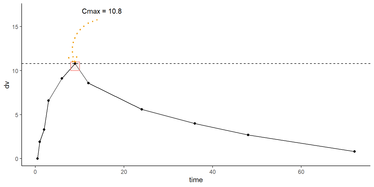
6  1  9.0 100 10.8   cp    0 66.7  50 male low wt old age
summary(war_pk)
       id           time             amt              dv          dvid    
 9      : 17   Min.   :  0.50   Min.   : 60.0   Min.   : 0.000   cp :251  
 1      : 11   1st Qu.: 18.00   1st Qu.: 88.5   1st Qu.: 3.200   pca:  0  
 3      : 11   Median : 36.00   Median :105.0   Median : 6.100            
 8      : 11   Mean   : 50.07   Mean   :103.1   Mean   : 6.412            
 15     : 11   3rd Qu.: 72.00   3rd Qu.:117.0   3rd Qu.: 8.900            
 5      : 10   Max.   :120.00   Max.   :153.0   Max.   :17.600            
 (Other):180                                                              
      evid         wt              age            sex          wt_cat   
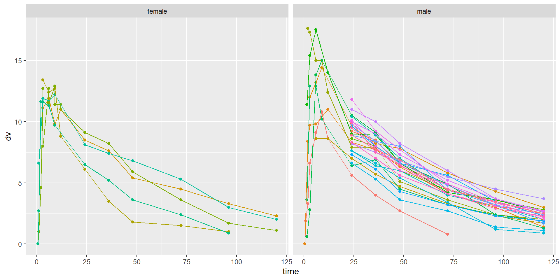
 Min.   :0   Min.   : 40.00   Min.   :21.00   female: 57   low wt :133  
 1st Qu.:0   1st Qu.: 59.00   1st Qu.:23.00   male  :194   high wt:118  
 Median :0   Median : 70.00   Median :31.00                             
 Mean   :0   Mean   : 68.71   Mean   :32.47                             
 3rd Qu.:0   3rd Qu.: 78.00   3rd Qu.:40.00                             
 Max.   :0   Max.   :102.00   Max.   :63.00                             
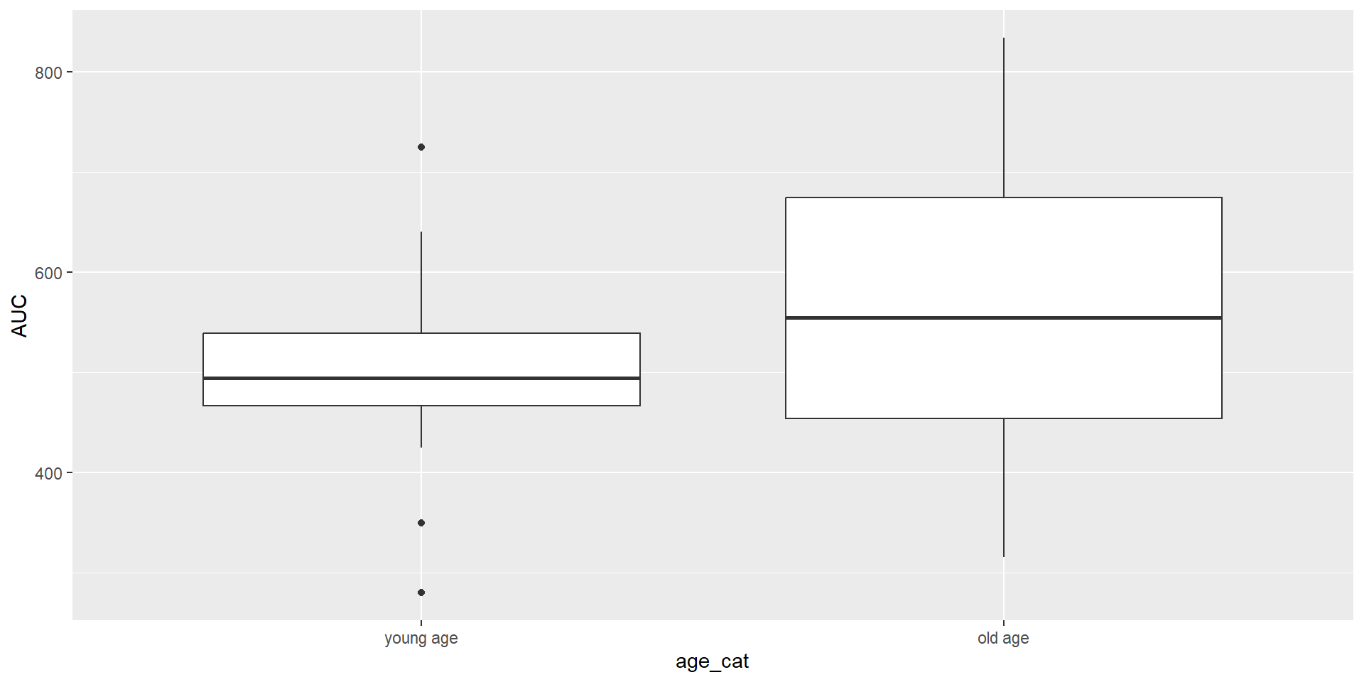
                                                                        
      age_cat   
 young age:123  
 old age  :128  


head(war_pd)
  id time amt dv dvid evid   wt age  sex wt_cat age_cat
1  1   24 100 44  pca    0 66.7  50 male low wt old age
2  1   36 100 27  pca    0 66.7  50 male low wt old age
3  1   48 100 28  pca    0 66.7  50 male low wt old age
4  1   72 100 31  pca    0 66.7  50 male low wt old age
5  1   96 100 60  pca    0 66.7  50 male low wt old age
6  1  120 100 65  pca    0 66.7  50 male low wt old age
summary(war_pd)
       id           time             amt              dv         dvid    
 3      :  8   Min.   :  0.00   Min.   : 60.0   Min.   :  9.0   cp :  0  
 4      :  8   1st Qu.: 24.00   1st Qu.: 90.0   1st Qu.: 20.0   pca:232  
 5      :  8   Median : 48.00   Median :105.0   Median : 28.0            
 6      :  8   Mean   : 61.45   Mean   :104.7   Mean   : 37.5            
 8      :  8   3rd Qu.: 96.00   3rd Qu.:120.0   3rd Qu.: 42.0            
 9      :  8   Max.   :144.00   Max.   :153.0   Max.   :100.0            
 (Other):184                                                             
      evid         wt              age           sex          wt_cat   
 Min.   :0   Min.   : 40.00   Min.   :21.0   female: 39   low wt :118  
 1st Qu.:0   1st Qu.: 60.00   1st Qu.:22.0   male  :193   high wt:114  
 Median :0   Median : 70.00   Median :28.0                             
 Mean   :0   Mean   : 69.79   Mean   :31.3                             
 3rd Qu.:0   3rd Qu.: 80.00   3rd Qu.:36.0                             
 Max.   :0   Max.   :102.00   Max.   :63.0                             
                                                                       
      age_cat   
 young age:129  
 old age  :103  


head(war_exposure)
  id     AUC   wt age    sex  wt_cat age_cat
1  1 315.525 66.7  50   male  low wt old age
2  2 492.000 66.7  50   male  low wt old age
3  3 665.600 66.7  31   male  low wt old age
4  4 834.000 80.0  40   male high wt old age
5  5 669.450 40.0  46 female  low wt old age
6  6 495.000 75.3  43   male high wt old age
summary(war_exposure)
       id          AUC              wt              age           sex    
 1      : 1   Min.   :279.6   Min.   : 40.00   Min.   :21.0   female: 5  
 2      : 1   1st Qu.:456.8   1st Qu.: 61.50   1st Qu.:22.0   male  :27  
 3      : 1   Median :500.1   Median : 71.65   Median :27.5              
 4      : 1   Mean   :528.9   Mean   : 70.00   Mean   :31.0              
 5      : 1   3rd Qu.:608.3   3rd Qu.: 78.50   3rd Qu.:36.0              
 6      : 1   Max.   :834.0   Max.   :102.00   Max.   :63.0              
 (Other):26                                                              
     wt_cat        age_cat  
 low wt :16   young age:18  
 high wt:16   old age  :14  


There is little to no interplay between different visualization approaches in R.

ggplot2

The Grammar of Graphics

  • You must have at least one geometric layer to see a plot
  • You can add as many geometric layers
  • Order matters!
ggplot(data = <Data.Frame, tibble ...>,  mapping = aes(<MAP VARIABLES FROM DATAFRAME>))+ 
  <GEOMETRIC_LAYER>  + 
  <STATS_LAYER> +
  <FACETING> + 
  <COORDIATE> + 
  <POSITION> + 
  <SCALE;LIMITS> + 
  <ANNOTATE>+
  <THEME>

library(ggplot2)

ggplot(data = war_exposure, aes(x = age_cat,  y= AUC))+ 
  geom_boxplot()

ggplot(war_pk, aes(time, dv, color = id)) + 
  geom_point() + 
  geom_line() 

ggplot2 faceting

  • faceting is a way to create multiple plots based on variable(s)
  • facet_wrap() Crosses the variables in a single row or column
  • facet_grid() Forms a matrix of panels defined by row and column faceting variables. Better if one variable.
  • Faceting has formula syntax:
    • facet_*(.~var1): var1 on the x-axis
    • facet_*(var1~.): var1 on the y-axis
    • facet_*(var1+var2+var3~var1+var2+var3)

ggplot(war_pk, aes(time, dv, color = id)) + 
  geom_point() + 
  geom_line() +
  facet_grid(.~sex) + 
  theme(legend.position = "none")

ggplot(war_pk, aes(time, dv)) + 
  geom_point() + 
  geom_line() +
  facet_wrap(.~id) + 
  theme(legend.position = "none")

Exercise 1

  • Use war_pk data
  • map time on x-axis, dv on y-axis and color to id
  • try both facet_wrap and facet grid for wt_cat~sex
  • which once is better in this case?
05:00

ggplot(war_pk, aes(time, dv, color = id)) + 
  geom_point() + 
  geom_line() +
  facet_wrap(wt_cat~sex) + 
  theme(legend.position = "none")

Exercise 2

  • Use war_pd data
  • map time on x-axis, dv on y-axis and color to id
  • facet_grid by wt_cat on y-axis and combination of sex and age_cat on x-axis
  • pass margin = TRUE
05:00

ggplot(war_pd, aes(time, dv, color = id)) + 
  geom_point() + 
  geom_line() +
  facet_grid(wt_cat~sex+age_cat, margin = TRUE) + 
  theme(legend.position = "none")

Changing global aesthetics

ggplot(war_pk, aes(time, dv)) + 
  geom_line(color = "red") + 
  geom_line(data = war_pd, aes(time, dv/4), color = "blue") +
  facet_wrap(.~id)  + 
  scale_y_continuous(sec.axis = sec_axis(~.*4), name = "prothrombin complex activity (PCA)" ) +
  labs(x = "Concentration", y = "Time")

Exercise 3

  • Use the provided dataframe points to create the following figure.
  • You will need geom_polygon for that. Map xand y. choose the appropriate color and fill.
  • Use annotate to create the annotation text and curve.
05:00

filter <- war_pk |> filter(id == 1)
cmax <- max(filter$dv) # 10.8
tmax <- filter$time[filter$dv == cmax] # 9
points <- data.frame(x = c(8, 10, 10, 8), y = c(10, 10, 11, 11))

ggplot(filter, aes(time, dv)) +
  geom_point() + 
  geom_line() + 
  geom_polygon(data = points  , aes(x , y, fill = "grey", col = "red"), 
               alpha = 0.1) + 
  annotate('curve', x = tmax+5, y = cmax+5, xend = tmax, yend=cmax, 
           curvature = 0.5, arrow = arrow(length = unit(0.2, 'in')), 
           linewidth = 1, linetype = "dotted", color = "orange2") +
  annotate('text', x = tmax+6, y = cmax+6, label = paste("Cmax =", cmax)) +
  geom_hline(yintercept = cmax, linetype = "dashed") +
  theme_classic() +
  theme(legend.position = "none")

Fancy interactive ploting with plotly

plotly

  • plotly offers interactive javascript plots
library(plotly)
plot_ly(data = war_pk, x = ~time, y = ~dv, color = ~id, 
        type = "scatter", mode = "lines+markers") |>
    layout(title = "PK Warfarin", xaxis = list(title = "Time"), 
         yaxis = list(title = "Concentration"),
         autosize = F, width = 700, height = 400)

# custom hover 
plot_ly(data = war_pk, x = ~time, y = ~dv, color = ~id, 
        type = "scatter", mode = "lines+markers") |>
  layout(title = "PK Warfarin", xaxis = list(title = "Time"), 
         yaxis = list(title = "Concentration"),
         autosize = F, width = 700, height = 400) |>
  add_trace(text = ~paste("ID: ", id, "<br>Time: ", time, 
                          "<br>Conc.: ", dv, 
                          "<br>Age:", age, "<br>Wt:" , wt))

Exercise 4

Repeat for PD data with plotly

  • data war_pkpd
  • map x to cp and y to pca
  • modify the text trace to include all relevant information; age, wt …etc.
05:00
plot_ly(data = war_pkpd, x = ~cp, y = ~pca, color = ~id, type = "scatter", mode = "lines+markers") |>
  layout(title = "PD Warfarin", xaxis = list(title = "Concentration"), yaxis = list(title = "prothrombin complex activity (PCA)")) |>
  add_trace(text = ~paste("ID: ", id, "<br>Concentration: ", cp, "<br>PCA: ", pca, "<br>Age:", age, "<br>Wt:" , wt)) |> 
  layout(autosize = F, width = 700, height = 400)

3D plot

plot_ly(iris,x=~Petal.Width,y=~Sepal.Width,z=~Petal.Length, color = ~Species)

Subplots

Merge multiple plots together

# figure a
a <- plot_ly(y = ~rnorm(50), type = "box", name = "trace 1")

# figure b 
pal <- c("red", "blue", "green")
pal <- setNames(pal, c("virginica", "setosa", "versicolor"))
b <-  plot_ly(data = iris, x = ~Sepal.Length, y = ~Petal.Length, 
              color = ~Species, colors = pal)

# figure c
trace_5 <- rnorm(100, mean = 5)
trace_6 <- rnorm(100, mean = 0)
trace_7 <- rnorm(100, mean = -5)
x <- c(1:100)

data <- data.frame(x, trace_5, trace_6, trace_7)

c <- plot_ly(data, x = ~x, y = ~trace_5, name = 'trace 5', 
             type = 'scatter', mode = 'lines') 
c <- c |> add_trace(y = ~trace_6, name = 'trace 6', mode = 'lines+markers') 
c <- c |> add_trace(y = ~trace_7, name = 'trace 7', mode = 'markers')

subplot(list(a, b, c)) |> 
  layout(autosize = F, width = 800, height = 450)

Subplots

Exercise 5

05:00

create interactive boxplot of PK data war_pk for each: sex, age_cat, wt_cat

a <- plot_ly(war_pk,x = ~sex, y = ~dv, type = "box",showlegend = F)
b <- plot_ly(war_pk,x = ~age_cat, y = ~dv, type = "box",showlegend = F)
c <- plot_ly(war_pk,x = ~wt_cat, y = ~dv, type = "box",showlegend = F)
subplot(list(a,b,c)) 

Get things faster with purrr

purrr

  • The idea is to replace loops with a concise and readable function call.

    Source: Advanced R, Hadley Wickham

Basic Example

library(purrr)

map(select(war_pk, age, wt, dv),  
    \(x) {ggplot(war_pk, aes(x = x)) + geom_density()})

map(c("age_cat", "wt_cat", "sex"),  
    \(x) {ggplot(war_exposure, aes(x = .data[[x]], y = AUC)) + geom_boxplot()})

Save multiple ggplot2 plots

plots_list <- map(c("age_cat", "wt_cat", "sex"),  
                  \(x) {ggplot(war_exposure, aes(x = .data[[x]], y = AUC)) + geom_boxplot()})

walk2(c("age_cat", "wt_cat", "sex"), plots_list, 
      \(x,y) ggsave(filename = paste0(x, "boxplot.png"), plot = y,height = 7, width = 7))

Exercise 6

  • Create interactive grid plots for PK data war_pk split by ID using map()
05:00
map(split(war_pk, war_pk$id), \(x){
        plot_ly(data = x, x = ~time, y = ~dv, type = "scatter", 
                mode = "lines", name = ~id)
    }) |> 
    subplot(nrows = 5)

THANK YOU!